Evaluating KOMPUTE - Clinical Chemistry data
Coby Warkentin and Donghyung Lee
2023-07-03
- Load packages
- Preparing control phenotype
data
- Importing Clinical Chemistry Control Phenotype Dataset
- Visualizing measured phenotypes via a heatmap
- Exclude phenotypes with fewer than 20,000 observations
- Remove samples with fewer than 15 measured phenotypes
- Heapmap of filtered phenotypes
- Reforatting the dataset (long to wide)
- Visualizing phenotype distributions
- Rank Z transformation
- Conducting Principal Variance Component Analysis (PVCA)
- Batch effect removal using ComBat
- PVCA on ComBat residuals
- Computing phenotypic correlations
- Preparation of IMPC
summary statistics data
- Loading Clinical Chemistry summary stat (IMPCv16)
- Visualizing gene-phenotype pair duplicates
- Consolidating muliple z-scores of a gene-phenotype pair using Stouffer’s Method
- Generating Z-score matrix (reformatting)
- Visualization of Phenotype-Gene Coverage
- Distribution of Z-Scores Across Phenotypes
- Estimation of Genetic Correlation Matrix Using Z-Scores
- Comparison of Phenotypic Correlation and Genetic Correlation Among Phenotypes
- Correlation Analysis Between Genetic Correlation Matrices Using Mantel’s Test
- Evaluating the KOMPUTE Imputation Algorithm
Last updated: 2023-07-03
Checks: 7 0
Knit directory: komputeExamples/
This reproducible R Markdown analysis was created with workflowr (version 1.7.0.1). The Checks tab describes the reproducibility checks that were applied when the results were created. The Past versions tab lists the development history.
Great! Since the R Markdown file has been committed to the Git repository, you know the exact version of the code that produced these results.
Great job! The global environment was empty. Objects defined in the global environment can affect the analysis in your R Markdown file in unknown ways. For reproduciblity it’s best to always run the code in an empty environment.
The command set.seed(20230110) was run prior to running
the code in the R Markdown file. Setting a seed ensures that any results
that rely on randomness, e.g. subsampling or permutations, are
reproducible.
Great job! Recording the operating system, R version, and package versions is critical for reproducibility.
Nice! There were no cached chunks for this analysis, so you can be confident that you successfully produced the results during this run.
Great job! Using relative paths to the files within your workflowr project makes it easier to run your code on other machines.
Great! You are using Git for version control. Tracking code development and connecting the code version to the results is critical for reproducibility.
The results in this page were generated with repository version 0bd39c6. See the Past versions tab to see a history of the changes made to the R Markdown and HTML files.
Note that you need to be careful to ensure that all relevant files for
the analysis have been committed to Git prior to generating the results
(you can use wflow_publish or
wflow_git_commit). workflowr only checks the R Markdown
file, but you know if there are other scripts or data files that it
depends on. Below is the status of the Git repository when the results
were generated:
Ignored files:
    Ignored:    .DS_Store
    Ignored:    .Rhistory
    Ignored:    .Rproj.user/
    Ignored:    analysis/.DS_Store
    Ignored:    code/.DS_Store

Untracked files:
    Untracked:  analysis/kompute_test_app_v16.Rmd

Unstaged changes:
    Modified:   data/BC.imp.res.v16.RData
Note that any generated files, e.g. HTML, png, CSS, etc., are not included in this status report because it is ok for generated content to have uncommitted changes.
These are the previous versions of the repository in which changes were
made to the R Markdown (analysis/kompute_test_CC_v16.Rmd)
and HTML (docs/kompute_test_CC_v16.html) files. If you’ve
configured a remote Git repository (see ?wflow_git_remote),
click on the hyperlinks in the table below to view the files as they
were in that past version.
| File | Version | Author | Date | Message |
|---|---|---|---|---|
| Rmd | 0bd39c6 | statsleelab | 2023-07-03 | typo fix |
| html | b343ff3 | statsleelab | 2023-07-03 | svd mc added |
| Rmd | dbdfbca | statsleelab | 2023-07-03 | svd mc added |
| html | 0ad952c | statsleelab | 2023-06-23 | kompute function input format changed |
| Rmd | fbd0f5c | statsleelab | 2023-06-23 | kompute input format changed |
| html | dcb3b0d | statsleelab | 2023-06-21 | pheno.cor added |
| Rmd | e7a365f | statsleelab | 2023-06-21 | pheno.cor added |
| html | 9b680ec | statsleelab | 2023-06-20 | doc updated |
| Rmd | d343f6a | statsleelab | 2023-06-20 | doc updated |
| html | d56cc7a | statsleelab | 2023-06-19 | Build site. |
| html | f4e1ab9 | statsleelab | 2023-01-10 | v16 update |
| Rmd | 7685a09 | statsleelab | 2023-01-10 | first commit |
| html | 7685a09 | statsleelab | 2023-01-10 | first commit |
Load packages
rm(list=ls())
knitr::opts_chunk$set(message = FALSE, warning = FALSE)

library(data.table)
library(dplyr)
library(reshape2)
library(ggplot2)
library(tidyr) #spread
library(RColorBrewer)
library(circlize)
library(ComplexHeatmap)
Preparing control phenotype data
Importing Clinical Chemistry Control Phenotype Dataset
CC.data <- readRDS("data/CC.data.rds")
#dim(CC.data)
Visualizing measured phenotypes via a heatmap
The heatmap below presents a visualization of the phenotypic measurements taken for each control mouse. The columns represent individual mice, while the rows correspond to the distinct phenotypes measured.
mtest <- table(CC.data$proc_param_name_stable_id, CC.data$biological_sample_id)
mtest <-as.data.frame.matrix(mtest)
#dim(mtest)
if(FALSE){
nmax <-max(mtest)
library(circlize)
col_fun = colorRamp2(c(0, nmax), c("white", "red"))
col_fun(seq(0, nmax))
ht = Heatmap(as.matrix(mtest), cluster_rows = FALSE, cluster_columns = FALSE, show_column_names = F, col = col_fun,
             row_names_gp = gpar(fontsize = 8), name="Count")
draw(ht)
}
Exclude phenotypes with fewer than 20,000 observations
To maintain data quality and robustness, we will discard any phenotypes that have fewer than 20,000 recorded observations.
mtest <- table(CC.data$proc_param_name, CC.data$biological_sample_id)
#dim(mtest)
#head(mtest[,1:10])
mtest0 <- mtest>0
#head(mtest0[,1:10])
#rowSums(mtest0)
rmv.pheno.list <- rownames(mtest)[rowSums(mtest0)<20000]
#rmv.pheno.list
#dim(CC.data)
CC.data <- CC.data %>% filter(!(proc_param_name %in% rmv.pheno.list))
#dim(CC.data)
# number of phenotypes left
#length(unique(CC.data$proc_param_name))
Remove samples with fewer than 15 measured phenotypes
mtest <- table(CC.data$proc_param_name, CC.data$biological_sample_id)
#dim(mtest)
#head(mtest[,1:10])
mtest0 <- mtest>0
#head(mtest0[,1:10])
#summary(colSums(mtest0))
rmv.sample.list <- colnames(mtest)[colSums(mtest0)<15]
#length(rmv.sample.list)
#dim(CC.data)
CC.data <- CC.data %>% filter(!(biological_sample_id %in% rmv.sample.list))
#dim(CC.data)
# number of observations to use
#length(unique(CC.data$biological_sample_id))
Heapmap of filtered phenotypes
if(FALSE){
mtest <- table(CC.data$proc_param_name, CC.data$biological_sample_id)
dim(mtest)
mtest <-as.data.frame.matrix(mtest)
nmax <-max(mtest)
library(circlize)
col_fun = colorRamp2(c(0, nmax), c("white", "red"))
col_fun(seq(0, nmax))
pdf("~/Google Drive Miami/Miami_IMPC/output/measured_phenotypes_controls_after_filtering_CC.pdf", width = 10, height = 3)
ht = Heatmap(as.matrix(mtest), cluster_rows = FALSE, cluster_columns = FALSE, show_column_names = F, col = col_fun,
             row_names_gp = gpar(fontsize = 7), name="Count")
draw(ht)
dev.off()
}
Reforatting the dataset (long to wide)
We restructure our data from a long format to a wide one for further processing and analysis.
CC.mat <- CC.data %>%
  dplyr::select(biological_sample_id, proc_param_name, data_point, sex, phenotyping_center, strain_name) %>%
  ##consider weight or age in weeks
  arrange(biological_sample_id) %>%
  distinct(biological_sample_id, proc_param_name, .keep_all=TRUE) %>% ## remove duplicates, maybe mean() is better.
  spread(proc_param_name, data_point) %>%
  tibble::column_to_rownames(var="biological_sample_id")
head(CC.mat)
sex phenotyping_center strain_name CC_Alanine aminotransferase
21 male MRC Harwell 129S8/SvEv-Gpi1<c>/NimrH 85.9
22 male MRC Harwell 129S8/SvEv-Gpi1<c>/NimrH 110.9
24 male MRC Harwell 129S8/SvEv-Gpi1<c>/NimrH 32.1
25 male MRC Harwell 129S8/SvEv-Gpi1<c>/NimrH 33.7
26 male MRC Harwell 129S8/SvEv-Gpi1<c>/NimrH 37.2
27 male MRC Harwell 129S8/SvEv-Gpi1<c>/NimrH 39.7
CC_Albumin CC_Alkaline phosphatase CC_Alpha-amylase
21 25.3 90 759.2
22 26.9 86 844.3
24 26.5 103 822.9
25 26.2 81 799.9
26 28.4 95 810.5
27 27.3 93 821.4
CC_Aspartate aminotransferase CC_Calcium CC_Chloride CC_Creatinine
21 97.7 2.33 112 NA
22 114.7 2.41 113 NA
24 57.7 2.35 108 NA
25 64.0 2.35 110 NA
26 62.3 2.35 109 NA
27 58.3 2.37 109 NA
CC_Glucose CC_HDL-cholesterol CC_Iron CC_Phosphorus CC_Potassium CC_Sodium
21 8.46 NA 37.86 1.76 4.8 152
22 9.83 NA 39.78 1.82 5.7 153
24 8.36 NA 38.24 1.89 4.7 154
25 10.42 NA 36.28 2.10 4.8 153
26 9.79 NA 36.26 2.02 5.1 153
27 9.74 NA 38.30 1.57 4.5 153
CC_Total bilirubin CC_Total cholesterol CC_Total protein CC_Triglycerides
21 NA 3.27 50.6 1.04
22 NA 3.40 52.4 1.02
24 NA 3.63 52.4 1.43
25 NA 3.40 51.6 0.72
26 NA 3.53 51.9 1.15
27 NA 3.20 51.8 1.12
CC_Urea (Blood Urea Nitrogen - BUN)
21 NA
22 NA
24 NA
25 NA
26 NA
27 NA#dim(CC.mat)
#summary(colSums(is.na(CC.mat[,-1:-3])))Visualizing phenotype distributions
ggplot(melt(CC.mat), aes(x=value)) +
  geom_histogram() +
  facet_wrap(~variable, scales="free", ncol=5)+
  theme(strip.text.x = element_text(size = 6))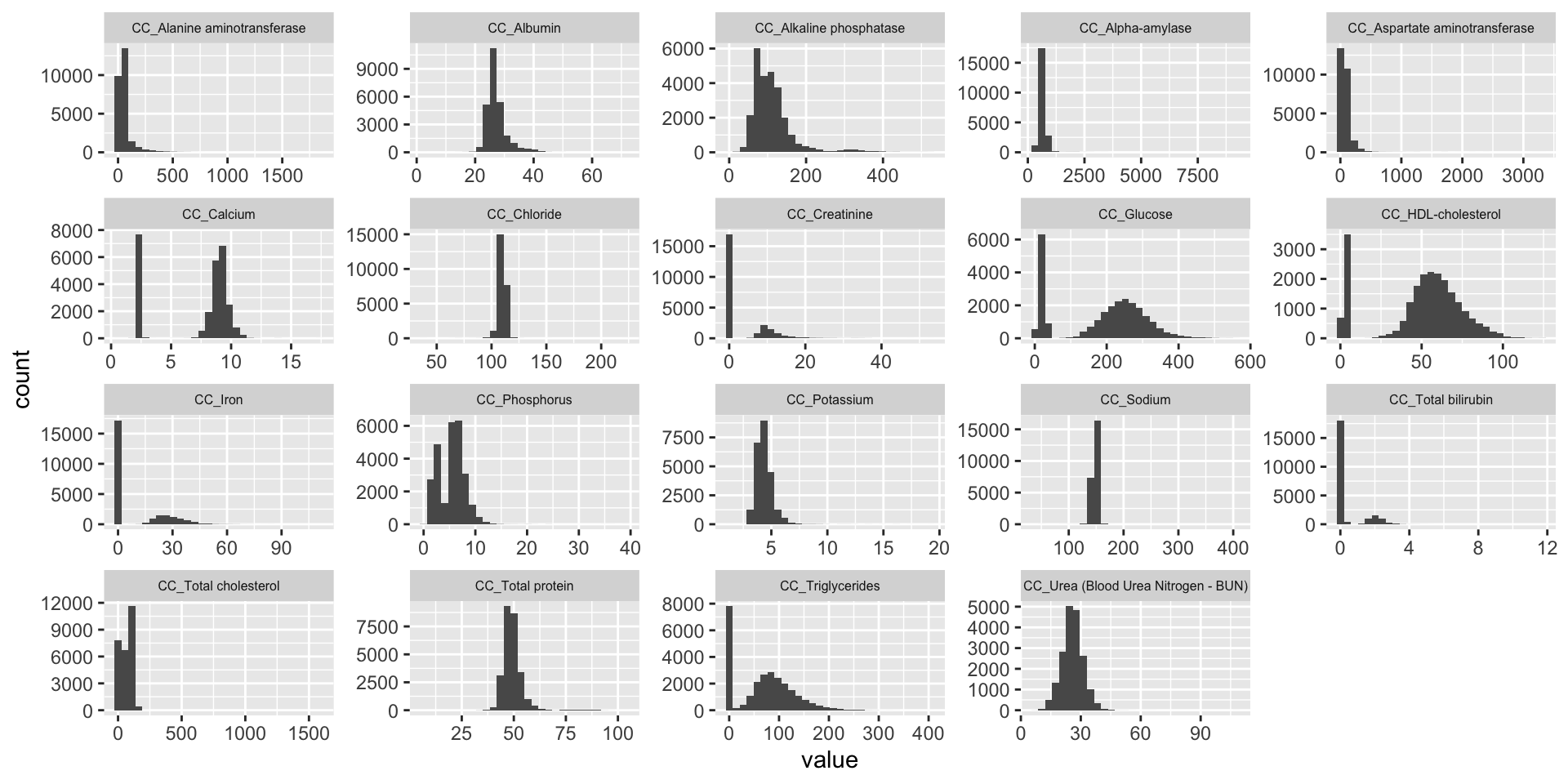
| Version | Author | Date |
|---|---|---|
| 7685a09 | statsleelab | 2023-01-10 |
Rank Z transformation
In this step, we conduct a rank Z transformation on the phenotype data to ensure that the data is normally distributed
library(RNOmni)
CC.mat.rank <- CC.mat
#dim(CC.mat.rank)
CC.mat.rank <- CC.mat.rank[complete.cases(CC.mat.rank),]
#dim(CC.mat.rank)

#dim(CC.mat)
CC.mat <- CC.mat[complete.cases(CC.mat),]
#dim(CC.mat)

CC.mat.rank <- cbind(CC.mat.rank[,1:3], apply(CC.mat.rank[,-1:-3], 2, RankNorm))
ggplot(melt(CC.mat.rank), aes(x=value)) +
  geom_histogram() +
  facet_wrap(~variable, scales="free", ncol=5)+
theme(strip.text.x = element_text(size = 6))![]()
| Version | Author | Date |
|---|---|---|
| 7685a09 | statsleelab | 2023-01-10 |
Conducting Principal Variance Component Analysis (PVCA)
In this step, we apply Principal Variance Component Analysis (PVCA) on the phenotype matrix data. PVCA is an approach that combines Principal Component Analysis (PCA) and Variance Component Analysis to quantify the proportion of total variance in the data attributed to each important covariate, in this case ‘sex’ and ‘phenotyping_center’.
First, we prepare our metadata which includes our chosen covariates. Any character variables in the metadata are then converted to factors. To avoid potential confounding, we check for associations between our covariates and drop ‘strain_name’ due to its strong association with ‘phenotyping_center’.
Next, we run PVCA on randomly chosen subsets of our phenotype data (for computational efficiency). Finally, we compute the average effect size across all random samples and visualize the results in a PVCA plot.
source("code/PVCA.R")

meta <- CC.mat.rank[,1:3] ## examining covariates sex, phenotyping_center, and strain_name
#head(meta)
#dim(meta)
#summary(meta) # variables are still characters
meta[sapply(meta, is.character)] <- lapply(meta[sapply(meta, is.character)], as.factor)
#summary(meta) # now all variables are converted to factors

chisq.test(meta[,1],meta[,2])
    Pearson's Chi-squared test

data:  meta[, 1] and meta[, 2]
X-squared = 0.032984, df = 2, p-value = 0.9836
chisq.test(meta[,2],meta[,3])
    Pearson's Chi-squared test

data:  meta[, 2] and meta[, 3]
X-squared = 14688, df = 6, p-value < 2.2e-16
meta<-meta[,-3] # phenotyping_center and strain_name strongly associated which could cause confounding in the PVCA analysis, so we drop 'strain_name'.
G <- t(CC.mat.rank[,-1:-3]) ## preparing the phenotype matrix data
set.seed(09302021)
# Perform PVCA for 10 random samples of size 1000 (more computationally efficient)
pvca.res <- matrix(nrow=10, ncol=3)
for (i in 1:10){
sample <- sample(1:ncol(G), 1000, replace=FALSE)
pvca.res[i,] <- PVCA(G[,sample], meta[sample,], threshold=0.6, inter=FALSE)
}
# Compute average effect size across the 10 random samples
pvca.means <- colMeans(pvca.res)
names(pvca.means) <- c(colnames(meta), "resid")
# Create PVCA plot
pvca.plot <- PlotPVCA(pvca.means, "PVCA of Phenotype Matrix Data")
pvca.plot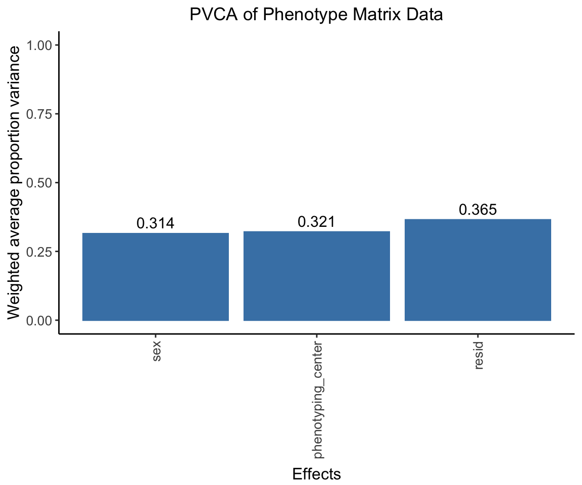
| Version | Author | Date |
|---|---|---|
| 7685a09 | statsleelab | 2023-01-10 |
png(file="docs/figure/figures.Rmd/pvca_CC_1_v16.png", width=600, height=350)
pvca.plot
dev.off()
quartz_off_screen
2 Batch effect removal using ComBat
We remove batch effects (the center effect) in the phenotype data set by using the ComBat method.
library(sva)
combat_komp = ComBat(dat=G, batch=meta$phenotyping_center, par.prior=TRUE, prior.plots=TRUE, mod=NULL)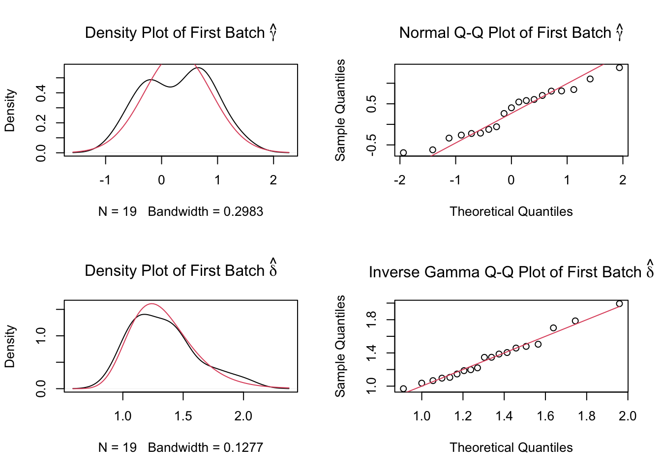
| Version | Author | Date |
|---|---|---|
| 7685a09 | statsleelab | 2023-01-10 |
#combat_komp[1:5,1:5]
#G[1:5,1:5] # for comparison, combat_komp is same form and same dimensions as G
PVCA on ComBat residuals
After using ComBat to account for batch effects, we perform a PVCA on the residuals. We expect to observe a significantly reduced effect from the phenotyping centers.
set.seed(09302021)
# Perform PVCA for 10 samples (more computationally efficient)
pvca.res.nobatch <- matrix(nrow=10, ncol=3)
for (i in 1:10){
  sample <- sample(1:ncol(combat_komp), 1000, replace=FALSE)
  pvca.res.nobatch[i,] <- PVCA(combat_komp[,sample], meta[sample,], threshold=0.6, inter=FALSE)
}

# Compute average effect size across samples
pvca.means.nobatch <- colMeans(pvca.res.nobatch)
names(pvca.means.nobatch) <- c(colnames(meta), "resid")

# Generate PVCA plot
pvca.plot.nobatch <- PlotPVCA(pvca.means.nobatch, "PVCA of Phenotype Matrix Data with Reduced Batch Effect")
pvca.plot.nobatch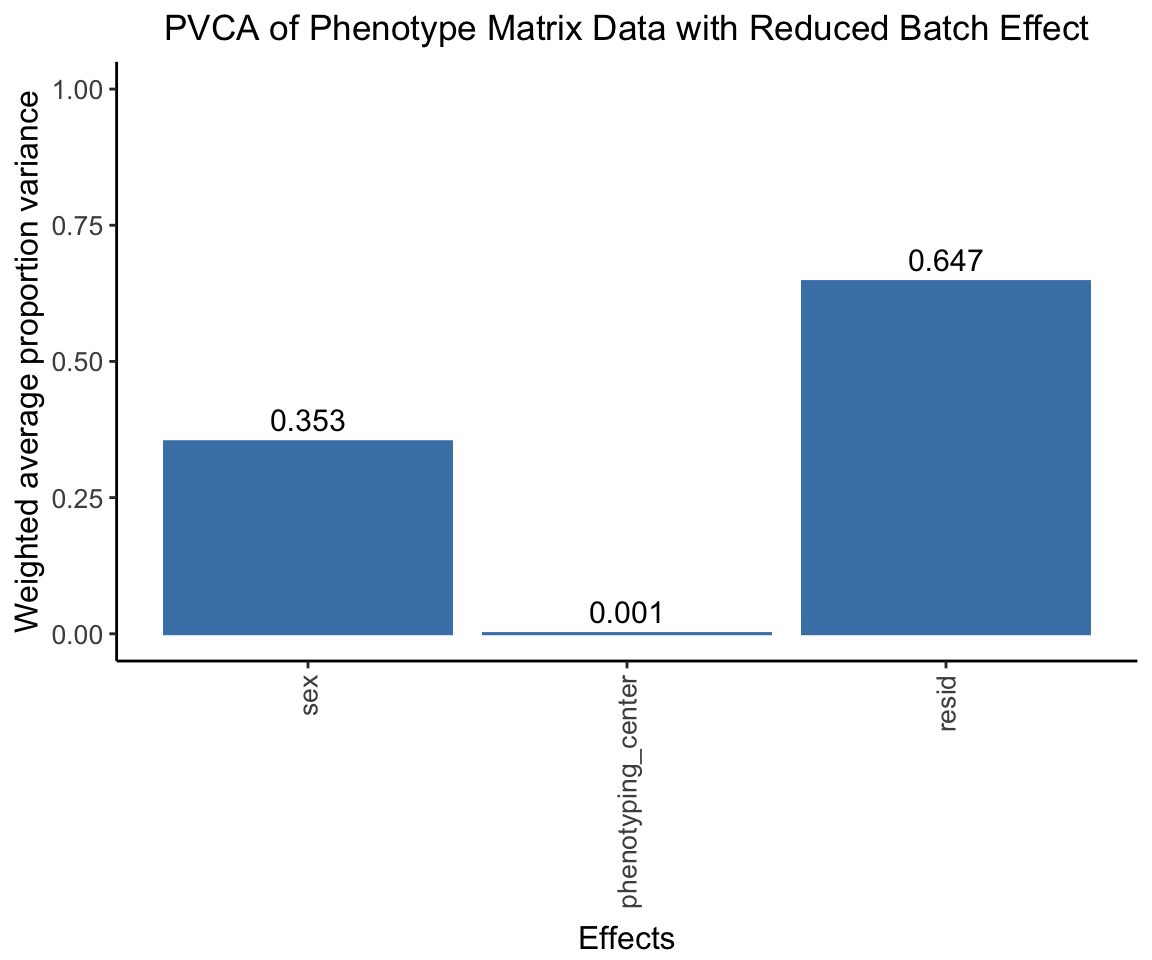
| Version | Author | Date |
|---|---|---|
| 7685a09 | statsleelab | 2023-01-10 |
png(file="docs/figure/figures.Rmd/pvca_CC_2_v16.png", width=600, height=350)
pvca.plot.nobatch
dev.off()
quartz_off_screen
2 Computing phenotypic correlations
We compute the phenotype correlations using different methods and compare them.
CC.cor.rank <- cor(CC.mat.rank[,-1:-3], use="pairwise.complete.obs") # pearson correlation coefficient
CC.cor <- cor(CC.mat[,-1:-3], use="pairwise.complete.obs", method="spearman") # spearman
CC.cor.combat <- cor(t(combat_komp), use="pairwise.complete.obs")
pheno.list <- rownames(CC.cor)

ht1 = Heatmap(CC.cor, show_column_names = F, row_names_gp = gpar(fontsize = 9), name="Spearm. Corr.")
draw(ht1)
ht2 = Heatmap(CC.cor.rank, show_column_names = F, row_names_gp = gpar(fontsize = 9), name="Corr. RankZ")
draw(ht2)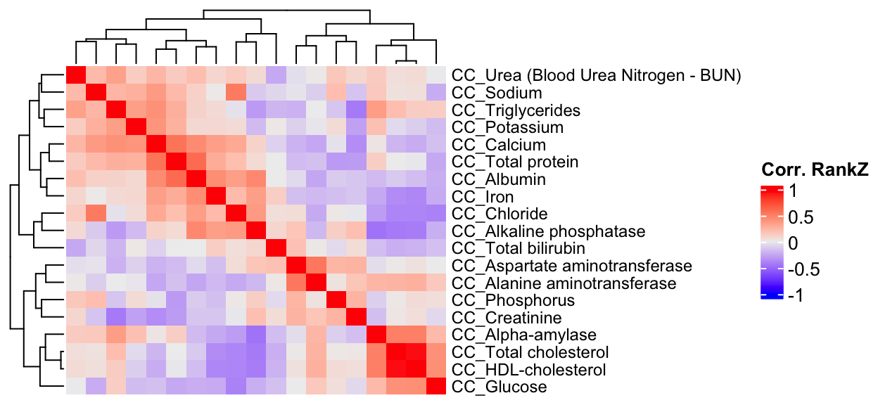
ht3 = Heatmap(CC.cor.combat, show_column_names = F, row_names_gp = gpar(fontsize = 9), name="Corr. ComBat")
draw(ht3)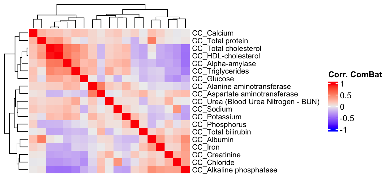
Preparation of IMPC summary statistics data
Loading Clinical Chemistry summary stat (IMPCv16)
CC.stat <- readRDS("data/CC.stat.v16.rds")
#dim(CC.stat)
table(CC.stat$parameter_name, CC.stat$procedure_name)
                                     CC
  Alanine aminotransferase         6312
  Albumin                          6312
  Alkaline phosphatase             6297
  Alpha-amylase                    3310
  Aspartate aminotransferase       6220
  Calcium                          6306
  Chloride                         3852
  Cholesterol ratio                2269
  Creatine kinase                  2744
  Creatinine                       5701
  Free fatty acids                 1595
  Fructosamine                     2301
  Glucose                          6276
  Glycerol                         1617
  HDL-cholesterol                  5148
  Iron                             4025
  LDL-cholesterol                  1871
  Magnesium                        1656
  Phosphorus                       6306
  Potassium                        4459
  Sodium                           3852
  Thyroxine                        1129
  Total bilirubin                  5841
  Total cholesterol                6301
  Total protein                    6278
  Triglycerides                    5473
  Urea (Blood Urea Nitrogen - BUN) 5523
#length(unique(CC.stat$marker_symbol)) #3983
#length(unique(CC.stat$allele_symbol)) #4152
#length(unique(CC.stat$proc_param_name)) #27, number of phenotypes in association statistics data set
#length(unique(CC.data$proc_param_name)) #19, number of phenotypes in final control data
pheno.list.stat <- unique(CC.stat$proc_param_name)
pheno.list.ctrl <- unique(CC.data$proc_param_name)
#sum(pheno.list.stat %in% pheno.list.ctrl)
#sum(pheno.list.ctrl %in% pheno.list.stat)
# Identifying common phenotypes between statistics and control data
common.pheno.list <- sort(intersect(pheno.list.ctrl, pheno.list.stat))
common.pheno.list [1] "CC_Alanine aminotransferase" "CC_Albumin"
[3] "CC_Alkaline phosphatase" "CC_Alpha-amylase"
[5] "CC_Aspartate aminotransferase" "CC_Calcium"
[7] "CC_Chloride" "CC_Creatinine"
[9] "CC_Glucose" "CC_HDL-cholesterol"
[11] "CC_Iron" "CC_Phosphorus"
[13] "CC_Potassium" "CC_Sodium"
[15] "CC_Total bilirubin" "CC_Total cholesterol"
[17] "CC_Total protein" "CC_Triglycerides"
[19] "CC_Urea (Blood Urea Nitrogen - BUN)"#length(common.pheno.list)
# Filtering summary statistics to contain only common phenotypes
#dim(CC.stat)
CC.stat <- CC.stat %>% filter(proc_param_name %in% common.pheno.list)
#dim(CC.stat)
#length(unique(CC.stat$proc_param_name))Visualizing gene-phenotype pair duplicates
mtest <- table(CC.stat$proc_param_name, CC.stat$marker_symbol)
mtest <-as.data.frame.matrix(mtest)
nmax <-max(mtest)
col_fun = colorRamp2(c(0, nmax), c("white", "red"))
#col_fun(seq(0, nmax))
ht = Heatmap(as.matrix(mtest), cluster_rows = FALSE, cluster_columns = FALSE, show_column_names = F, col = col_fun,
             row_names_gp = gpar(fontsize = 8), name="Count")
draw(ht)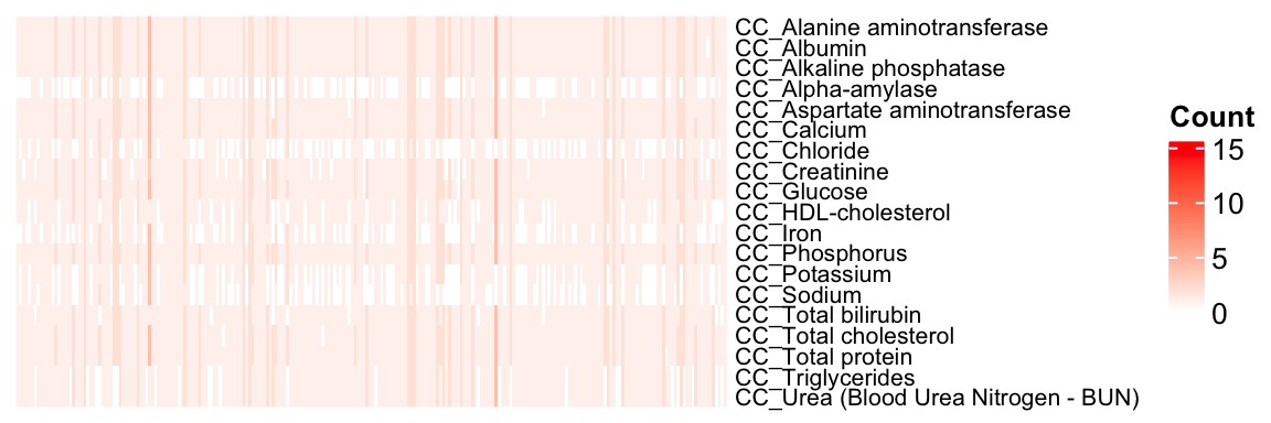
| Version | Author | Date |
|---|---|---|
| 7685a09 | statsleelab | 2023-01-10 |
Consolidating muliple z-scores of a gene-phenotype pair using Stouffer’s Method
## sum(z-score)/sqrt(# of zscore)
sumz <- function(z){ sum(z)/sqrt(length(z)) }
CC.z = CC.stat %>%
  dplyr::select(marker_symbol, proc_param_name, z_score) %>%
  na.omit() %>%
  group_by(marker_symbol, proc_param_name) %>%
  summarize(zscore = sumz(z_score)) ## combine z-scores
#dim(CC.z)
Generating Z-score matrix (reformatting)
# Function to convert NaN to NA
nan2na <- function(df){
  out <- data.frame(sapply(df, function(x) ifelse(is.nan(x), NA, x)))
  colnames(out) <- colnames(df)
  out
}

# Converting the long format of z-scores to a wide format matrix
CC.zmat = dcast(CC.z, marker_symbol ~ proc_param_name, value.var = "zscore",
             fun.aggregate = mean) %>% tibble::column_to_rownames(var="marker_symbol")
CC.zmat = nan2na(CC.zmat) #convert nan to na
#dim(CC.zmat)
Visualization of Phenotype-Gene Coverage
The heatmap illustrates tested (red) and untested (white) gene-phenotype pairs.
# Generate a matrix indicating where z-scores are present
id.mat <- 1*(!is.na(CC.zmat)) # multiply 1 to make this matrix numeric
#nrow(as.data.frame(colSums(id.mat)))
#dim(id.mat)

## heatmap of gene - phenotype (red: tested, white: untested)
ht = Heatmap(t(id.mat),
             cluster_rows = T, clustering_distance_rows ="binary",
             cluster_columns = T, clustering_distance_columns = "binary",
             show_row_dend = F, show_column_dend = F,  # do not show dendrogram
             show_column_names = F, col = c("white","red"),
             row_names_gp = gpar(fontsize = 10), name="Missing")
draw(ht)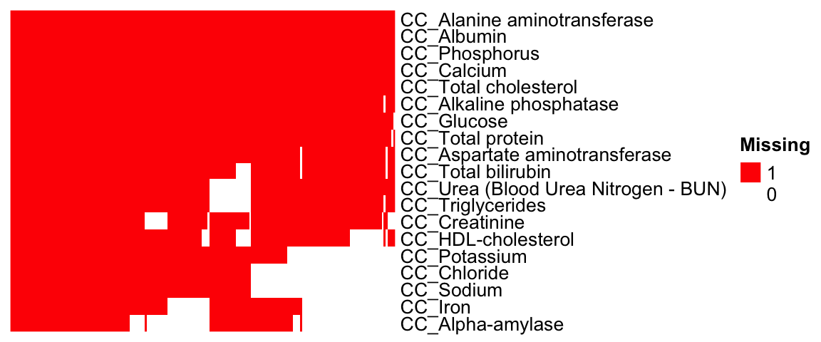
Distribution of Z-Scores Across Phenotypes
The histogram presents the distribution of association Z-scores for each phenotype.
ggplot(melt(CC.zmat), aes(x=value)) +
  geom_histogram() +
  facet_wrap(~variable, scales="free", ncol=5)+
  theme(strip.text.x = element_text(size = 6))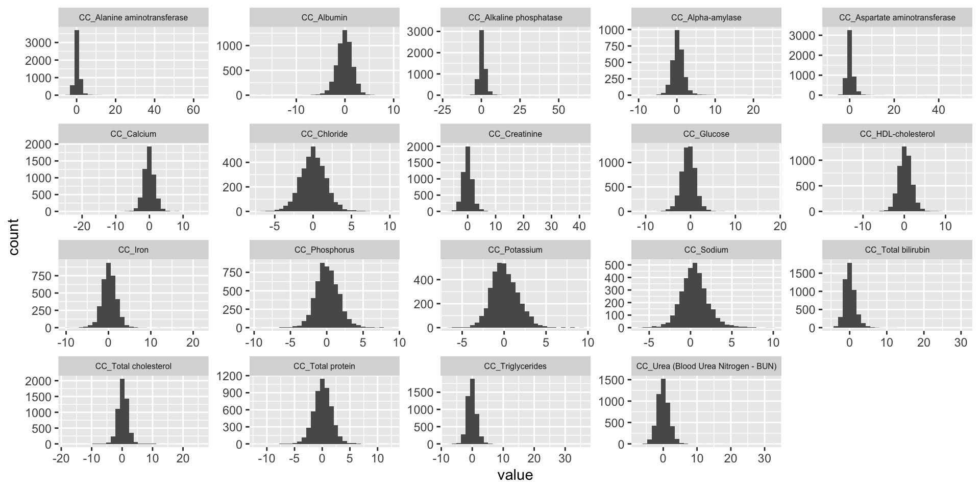
Estimation of Genetic Correlation Matrix Using Z-Scores
Here, we estimate the genetic correlations between phenotypes utilizing the association Z-score matrix.
# Select common phenotypes
CC.zmat <- CC.zmat[,common.pheno.list]
#dim(CC.zmat)

# Compute genetic correlations
CC.zcor = cor(CC.zmat, use="pairwise.complete.obs")

# Generate heatmap of the correlation matrix
ht = Heatmap(CC.zcor, cluster_rows = T, cluster_columns = T, show_column_names = F, #col = col_fun,
             row_names_gp = gpar(fontsize = 10),
             name="Genetic Corr (Z-score)"
             )
draw(ht)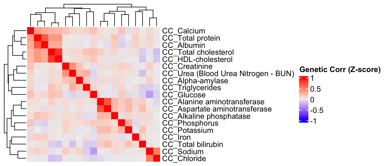
Comparison of Phenotypic Correlation and Genetic Correlation Among Phenotypes
We will compare the correlation matrix obtained from control mice phenotype data and the genetic correlation matrix estimated using association Z-scores. As depicted below, both correlation heatmaps show similar correlation patterns.
CC.cor.rank.fig <- CC.cor.rank[common.pheno.list,common.pheno.list]
CC.cor.fig <- CC.cor[common.pheno.list,common.pheno.list]
CC.cor.combat.fig <- CC.cor.combat[common.pheno.list, common.pheno.list]
CC.zcor.fig <- CC.zcor


ht = Heatmap(CC.cor.rank.fig, cluster_rows = TRUE, cluster_columns = TRUE, show_column_names = F, #col = col_fun,
              show_row_dend = F, show_column_dend = F,  # do not show dendrogram
             row_names_gp = gpar(fontsize = 8), column_title="Phenotype Corr (RankZ, Pearson)", column_title_gp = gpar(fontsize = 8),
             name="Corr")
pheno.order <- row_order(ht)
#draw(ht)

CC.cor.rank.fig <- CC.cor.rank.fig[pheno.order,pheno.order]
ht1 = Heatmap(CC.cor.rank.fig, cluster_rows = FALSE, cluster_columns = FALSE, show_column_names = F, #col = col_fun,
              show_row_dend = F, show_column_dend = F,  # do not show dendrogram
             row_names_gp = gpar(fontsize = 8), column_title="Phenotype Corr (RankZ, Pearson)", column_title_gp = gpar(fontsize = 8),
             name="Corr")
CC.cor.fig <- CC.cor.fig[pheno.order,pheno.order]
ht2 = Heatmap(CC.cor.fig, cluster_rows = FALSE, cluster_columns = FALSE, show_column_names = F, #col = col_fun,
             row_names_gp = gpar(fontsize = 8), column_title="Phenotype Corr (Spearman)", column_title_gp = gpar(fontsize = 8),
             name="Corr")
CC.cor.combat.fig <- CC.cor.combat.fig[pheno.order,pheno.order]
ht3 = Heatmap(CC.cor.combat.fig, cluster_rows = FALSE, cluster_columns = FALSE, show_column_names = F, #col = col_fun,
             row_names_gp = gpar(fontsize = 8), column_title="Phenotype Corr (Combat, Pearson)", column_title_gp = gpar(fontsize = 8),
             name="Corr")
CC.zcor.fig <- CC.zcor.fig[pheno.order,pheno.order]
ht4 = Heatmap(CC.zcor.fig, cluster_rows = FALSE, cluster_columns = FALSE, show_column_names = F, #col = col_fun,
             row_names_gp = gpar(fontsize = 8), column_title="Genetic Corr  (Pearson)", column_title_gp = gpar(fontsize = 8),
             name="Corr"
             )
draw(ht1+ht2+ht3+ht4)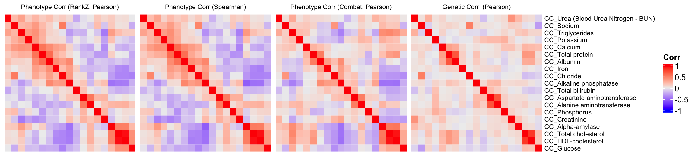
png(file="docs/figure/figures.Rmd/cors_CC.png", width=800, height=250)
draw(ht1+ht2+ht3+ht4)
dev.off()
quartz_off_screen
2 Correlation Analysis Between Genetic Correlation Matrices Using Mantel’s Test
To evaluate the correlation between different genetic correlation matrices, we apply Mantel’s test, which measures the correlation between two distance matrices.
####################
# Use Mantel test
# https://stats.idre.ucla.edu/r/faq/how-can-i-perform-a-mantel-test-in-r/
# install.packages("ade4")
library(ade4)
to.upper<-function(X) X[upper.tri(X,diag=FALSE)]

a1 <- to.upper(CC.cor.fig)
a2 <- to.upper(CC.cor.rank.fig)
a3 <- to.upper(CC.cor.combat.fig)
a4 <- to.upper(CC.zcor.fig)

plot(a4, a1)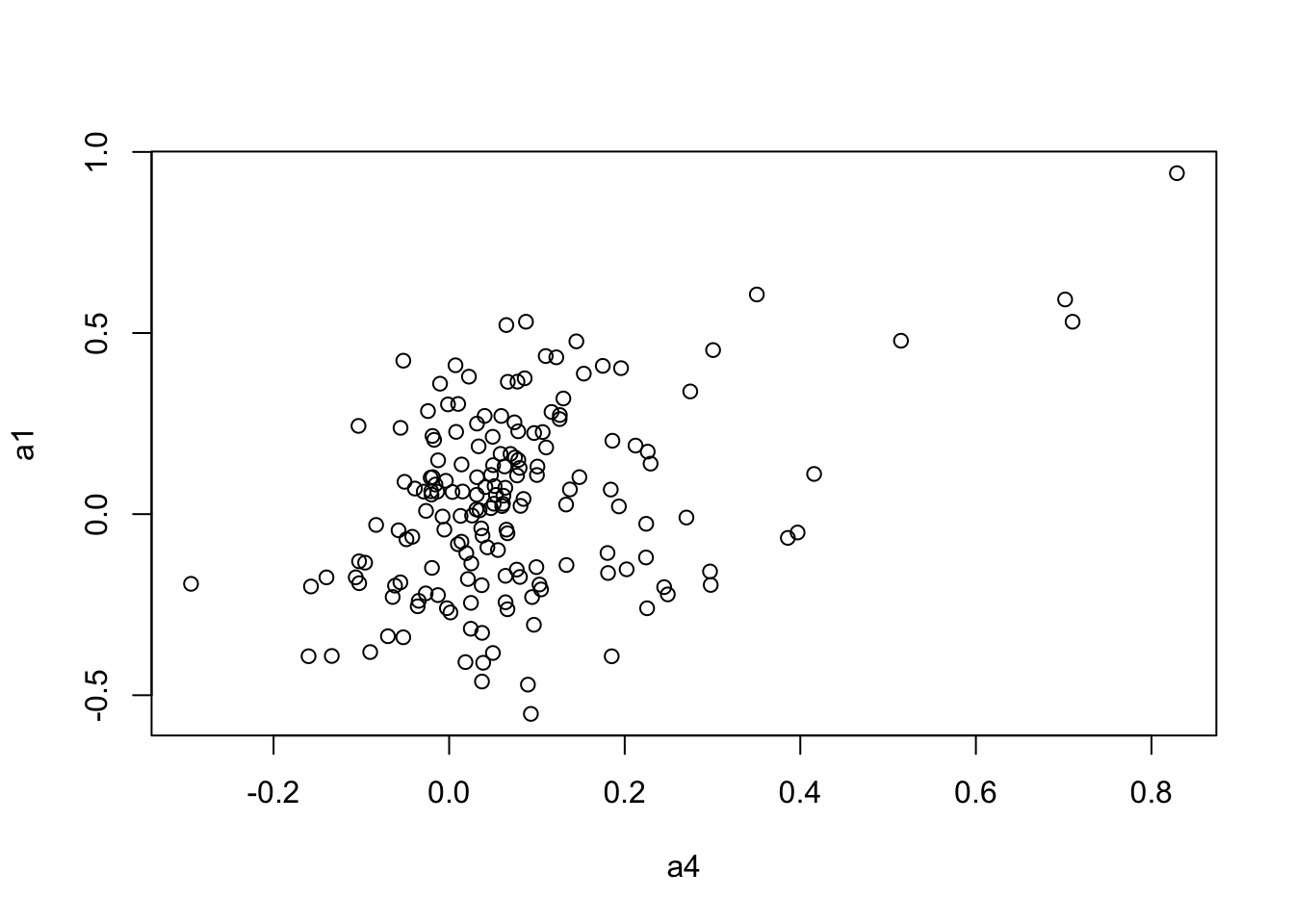
| Version | Author | Date |
|---|---|---|
| 9b680ec | statsleelab | 2023-06-20 |
plot(a4, a2)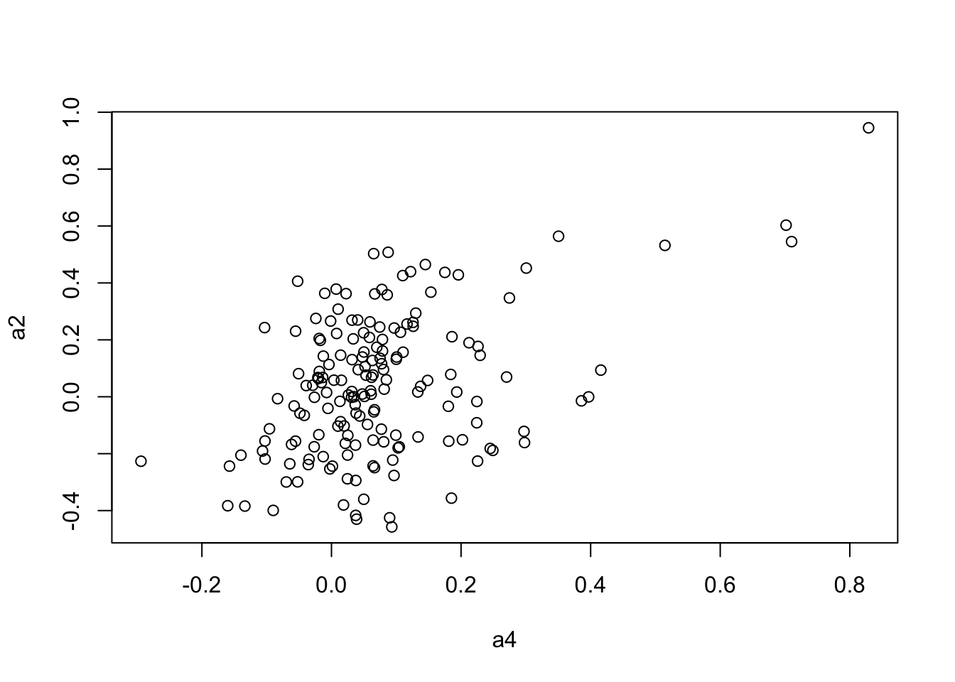
| Version | Author | Date |
|---|---|---|
| 9b680ec | statsleelab | 2023-06-20 |
plot(a4, a3)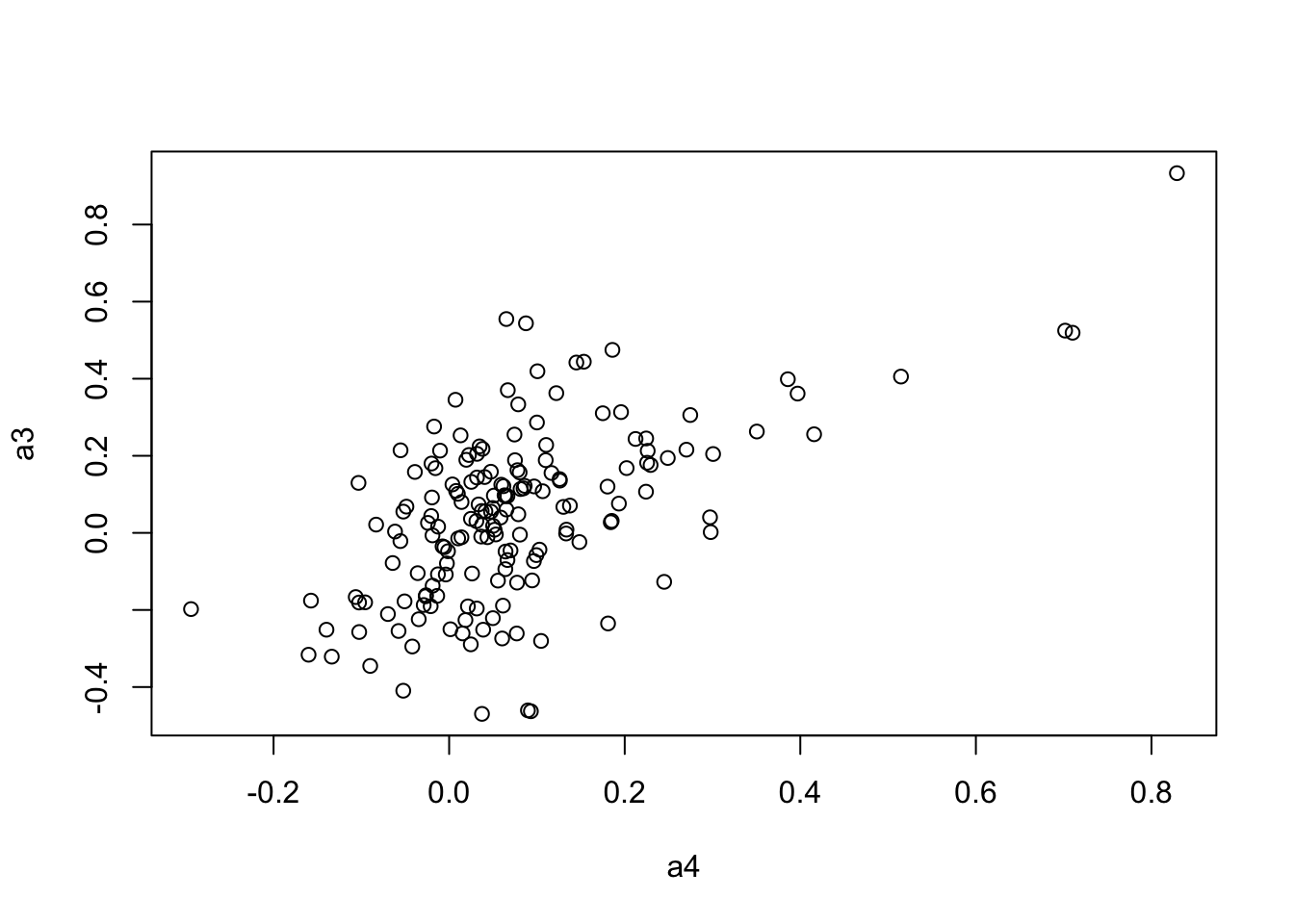
| Version | Author | Date |
|---|---|---|
| 9b680ec | statsleelab | 2023-06-20 |
mantel.rtest(as.dist(1-CC.cor.fig), as.dist(1-CC.zcor.fig), nrepet = 9999) #nrepet = number of permutationsMonte-Carlo test
Call: mantelnoneuclid(m1 = m1, m2 = m2, nrepet = nrepet)
Observation: 0.4065029
Based on 9999 replicates
Simulated p-value: 1e-04
Alternative hypothesis: greater
Std.Obs Expectation Variance
5.3342338350 0.0006783314 0.0057880553 mantel.rtest(as.dist(1-CC.cor.rank.fig), as.dist(1-CC.zcor.fig), nrepet = 9999)Monte-Carlo test
Call: mantelnoneuclid(m1 = m1, m2 = m2, nrepet = nrepet)
Observation: 0.4418449
Based on 9999 replicates
Simulated p-value: 1e-04
Alternative hypothesis: greater
Std.Obs Expectation Variance
5.775580172 0.001222770 0.005820245 mantel.rtest(as.dist(1-CC.cor.combat.fig), as.dist(1-CC.zcor.fig), nrepet = 9999)Monte-Carlo test
Call: mantelnoneuclid(m1 = m1, m2 = m2, nrepet = nrepet)
Observation: 0.5885487
Based on 9999 replicates
Simulated p-value: 1e-04
Alternative hypothesis: greater
Std.Obs Expectation Variance
7.818172131 -0.001408542 0.005694173 Evaluating the KOMPUTE Imputation Algorithm
Initializing the KOMPUTE Package
# Check if KOMPUTE is installed, if not, install it from GitHub using devtools
if(!"kompute" %in% rownames(installed.packages())){
  library(devtools)
  devtools::install_github("dleelab/kompute")
}
library(kompute)
Simulation study - Comparison of imputed vs measured z-score values
In this section, we conduct a simulation study to compare the performance of the KOMPUTE method with the measured gene-phenotype association z-scores. We randomly select some of these measured z-scores, mask them, and then use the KOMPUTE method to impute them. We then compare the imputed z-scores with the measured ones.
zmat <-t(CC.zmat)
dim(zmat)
[1] 19 5342# filter genes with less than 1 missing data point (na)
zmat0 <- is.na(zmat)
num.na<-colSums(zmat0)
#summary(num.na)
#dim(zmat)
#dim(zmat[,num.na<1])
#dim(zmat[,num.na<5])
#dim(zmat[,num.na<10])
# filter genes with less than 1 missing data point (na)
zmat <- zmat[,num.na<1]
#dim(zmat)
# Set correlation method for phenotypes
#pheno.cor <- CC.cor.fig
#pheno.cor <- CC.cor.rank.fig
pheno.cor <- CC.cor.combat.fig
#pheno.cor <- CC.zcor.fig
zmat <- zmat[rownames(pheno.cor),,drop=FALSE]
#rownames(zmat)
#rownames(pheno.cor)
#colnames(pheno.cor)
npheno <- nrow(zmat)
## calculate the percentage of missing Z-scores in the original data
100*sum(is.na(zmat))/(nrow(zmat)*ncol(zmat)) # 0%[1] 0nimp <- 1000 # # of missing/imputed Z-scores
set.seed(2222)
## find index of all measured zscores
all.i <- 1:(nrow(zmat)*ncol(zmat))
measured <- as.vector(!is.na(as.matrix(zmat)))
measured.i <- all.i[measured]
## mask 2000 measured z-scores
mask.i <- sort(sample(measured.i, nimp))
org.z = as.matrix(zmat)[mask.i]
zvec <- as.vector(as.matrix(zmat))
zvec[mask.i] <- NA
zmat.imp <- matrix(zvec, nrow=npheno)
rownames(zmat.imp) <- rownames(zmat)Run KOMPUTE method
kompute.res <- kompute(t(zmat.imp), pheno.cor, 0.01)

# Compare measured vs imputed z-scores
length(org.z)
[1] 1000imp.z <- as.matrix(t(kompute.res$zmat))[mask.i]
imp.info <- as.matrix(t(kompute.res$infomat))[mask.i]
# Create a dataframe with the original and imputed z-scores and the information of imputed z-scores
imp <- data.frame(org.z=org.z, imp.z=imp.z, info=imp.info)
#dim(imp)
imp <- imp[complete.cases(imp),]
imp <- subset(imp, info>=0 & info <= 1)
#dim(imp)
cor.val <- round(cor(imp$imp.z, imp$org.z), digits=3)
#cor.val
g <- ggplot(imp, aes(x=imp.z, y=org.z)) +
geom_point() +
labs(title=paste0("IMPC CC Data, Cor=",cor.val),
x="Imputed Z-scores", y = "Measured Z-scores") +
theme_minimal()
g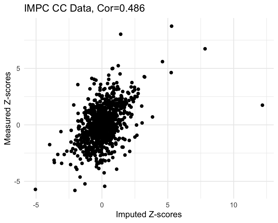
# Set a cutoff for information content and filter the data accordingly
info.cutoff <- 0.8
imp.sub <- subset(imp, info>info.cutoff)
#dim(imp.sub)
#summary(imp.sub$imp.z)
#summary(imp.sub$info)

cor.val <- round(cor(imp.sub$imp.z, imp.sub$org.z), digits=3)
#cor.val
g <- ggplot(imp.sub, aes(x=imp.z, y=org.z, col=info)) +
    geom_point() +
    labs(title=paste0("IMPC Behavior Data (CC), Info>", info.cutoff, ", Cor=",cor.val),
      x="Imputed Z-scores", y = "Measured Z-scores", col="Info") +
    theme_minimal()
g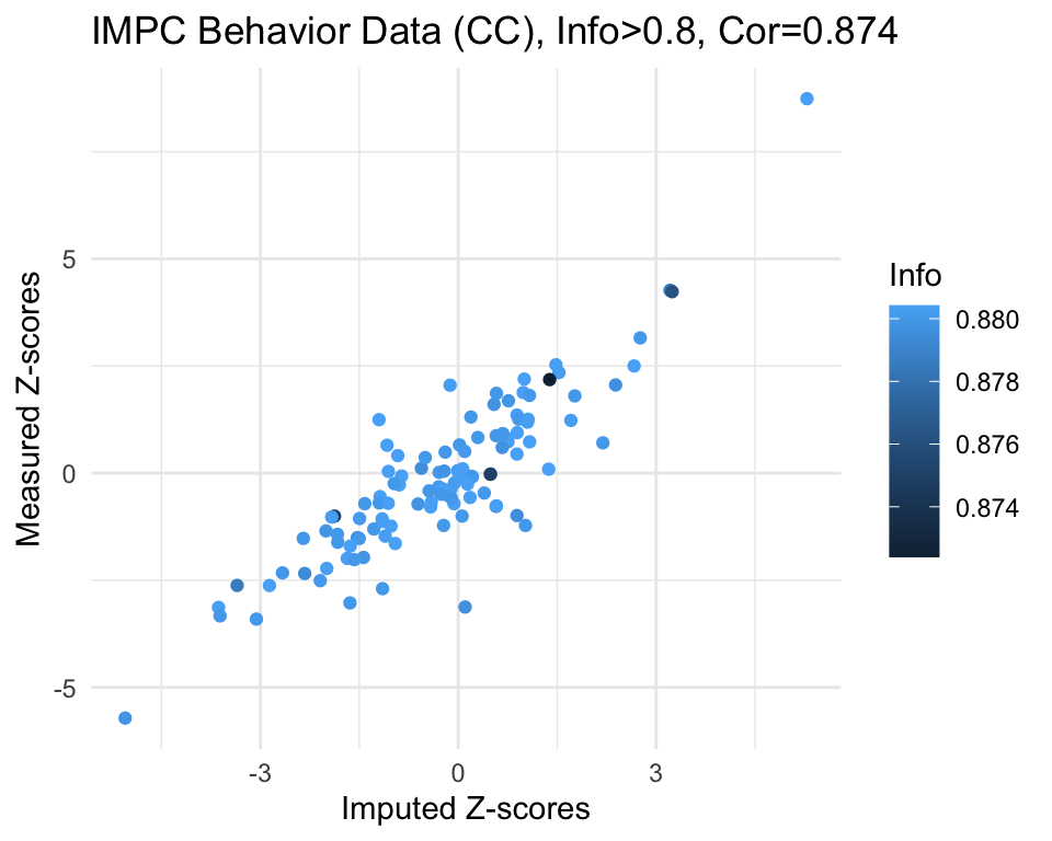
# save plot
png(file="docs/figure/figures.Rmd/sim_results_CC_v16.png", width=600, height=350)
g
dev.off()
quartz_off_screen
2 # Part 2 of Figure 2
fig2.2 <- ggplot(imp.sub, aes(x=imp.z, y=org.z, col=info)) +
geom_point() +
labs(title="Clinical Chemistry",
x="Imputed Z-scores", y = "", col="Info") +
scale_x_continuous(limits=c(-9,9), breaks=c(seq(-9,9,3)), minor_breaks = NULL) +
scale_y_continuous(limits=c(-9,9), breaks=c(seq(-9,9,3))) +
scale_color_gradient(limits=c(0.8,1), low="#98cdf9", high="#084b82") +
theme_bw() +
theme(legend.position="none", plot.title=element_text(hjust=0.5))
save(fig2.2, file="docs/figure/figures.Rmd/sim_CC_v16.rdata")Run SVD Matrix Completion method
# load SVD Matrix Completion function
source("code/svd_impute.R")
r <- 6
mc.res <- svd.impute(zmat.imp, r)

# Compare measured vs imputed z-scores
length(org.z)
[1] 1000imp.z <- mc.res[mask.i]
#plot(imp.z, org.z)
#cor(imp.z, org.z)
# Create a dataframe with the original and imputed z-scores and the information of imputed z-scores
imp2 <- data.frame(org.z=org.z, imp.z=imp.z)
#dim(imp2)
imp2 <- imp2[complete.cases(imp2),]
cor.val <- round(cor(imp2$imp.z, imp2$org.z), digits=3)
#cor.val
g <- ggplot(imp2, aes(x=imp.z, y=org.z)) +
geom_point() +
labs(title=paste0("IMPC CC Data, Cor=",cor.val),
x="Imputed Z-scores", y = "Measured Z-scores") +
theme_minimal()
g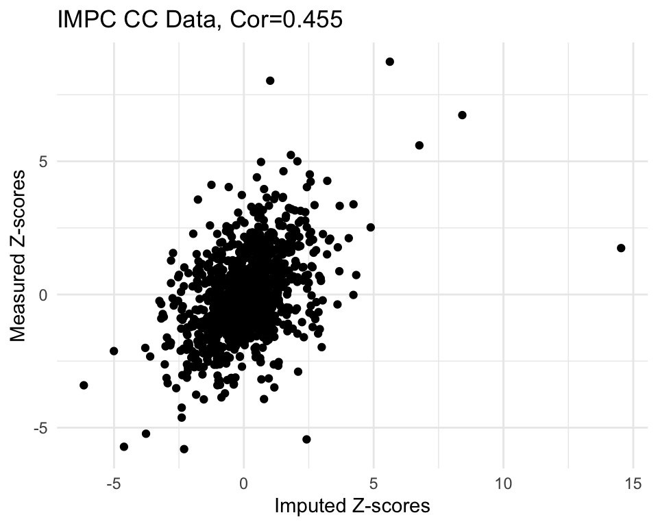
| Version | Author | Date |
|---|---|---|
| b343ff3 | statsleelab | 2023-07-03 |
Save imputation results
imp$method <- "KOMPUTE"
imp2$method <- "SVD-MC"
imp2$info <- NA
CC_Imputation_Result <- rbind(imp, imp2)
save(CC_Imputation_Result, file = "data/CC.imp.res.v16.RData")
Save z-score matrix and phenotype correlation matrix
plist <- sort(colnames(CC.zmat))
CC_Zscore_Mat <- as.matrix(CC.zmat[,plist])
save(CC_Zscore_Mat, file = "data/CC.zmat.v16.RData")

CC_Pheno_Cor <- pheno.cor[plist,plist]
save(CC_Pheno_Cor, file = "data/CC.pheno.cor.v16.RData")
sessionInfo()R version 4.2.1 (2022-06-23)
Platform: x86_64-apple-darwin17.0 (64-bit)
Running under: macOS Catalina 10.15.7
Matrix products: default
BLAS: /Library/Frameworks/R.framework/Versions/4.2/Resources/lib/libRblas.0.dylib
LAPACK: /Library/Frameworks/R.framework/Versions/4.2/Resources/lib/libRlapack.dylib
locale:
[1] en_US.UTF-8/en_US.UTF-8/en_US.UTF-8/C/en_US.UTF-8/en_US.UTF-8
attached base packages:
[1] grid stats graphics grDevices utils datasets methods
[8] base
other attached packages:
[1] kompute_0.1.0 ade4_1.7-20 sva_3.44.0
[4] BiocParallel_1.30.3 genefilter_1.78.0 mgcv_1.8-40
[7] nlme_3.1-158 lme4_1.1-31 Matrix_1.5-1
[10] RNOmni_1.0.1 ComplexHeatmap_2.12.1 circlize_0.4.15
[13] RColorBrewer_1.1-3 tidyr_1.2.0 ggplot2_3.4.1
[16] reshape2_1.4.4 dplyr_1.0.9 data.table_1.14.2
[19] workflowr_1.7.0.1
loaded via a namespace (and not attached):
[1] minqa_1.2.5 colorspace_2.1-0 rjson_0.2.21
[4] rprojroot_2.0.3 XVector_0.36.0 GlobalOptions_0.1.2
[7] fs_1.5.2 clue_0.3-62 rstudioapi_0.13
[10] farver_2.1.1 bit64_4.0.5 AnnotationDbi_1.58.0
[13] fansi_1.0.4 codetools_0.2-18 splines_4.2.1
[16] doParallel_1.0.17 cachem_1.0.6 knitr_1.39
[19] jsonlite_1.8.0 nloptr_2.0.3 annotate_1.74.0
[22] cluster_2.1.3 png_0.1-8 compiler_4.2.1
[25] httr_1.4.3 assertthat_0.2.1 fastmap_1.1.0
[28] limma_3.52.4 cli_3.6.0 later_1.3.0
[31] htmltools_0.5.3 tools_4.2.1 gtable_0.3.1
[34] glue_1.6.2 GenomeInfoDbData_1.2.8 Rcpp_1.0.10
[37] Biobase_2.56.0 jquerylib_0.1.4 vctrs_0.5.2
[40] Biostrings_2.64.0 iterators_1.0.14 xfun_0.31
[43] stringr_1.4.0 ps_1.7.1 lifecycle_1.0.3
[46] XML_3.99-0.10 edgeR_3.38.4 getPass_0.2-2
[49] MASS_7.3-58.1 zlibbioc_1.42.0 scales_1.2.1
[52] promises_1.2.0.1 parallel_4.2.1 yaml_2.3.5
[55] memoise_2.0.1 sass_0.4.2 stringi_1.7.8
[58] RSQLite_2.2.15 highr_0.9 S4Vectors_0.34.0
[61] foreach_1.5.2 BiocGenerics_0.42.0 boot_1.3-28
[64] shape_1.4.6 GenomeInfoDb_1.32.3 rlang_1.0.6
[67] pkgconfig_2.0.3 matrixStats_0.62.0 bitops_1.0-7
[70] evaluate_0.16 lattice_0.20-45 purrr_0.3.4
[73] labeling_0.4.2 bit_4.0.4 processx_3.7.0
[76] tidyselect_1.2.0 plyr_1.8.7 magrittr_2.0.3
[79] R6_2.5.1 IRanges_2.30.0 generics_0.1.3
[82] DBI_1.1.3 pillar_1.8.1 whisker_0.4
[85] withr_2.5.0 survival_3.3-1 KEGGREST_1.36.3
[88] RCurl_1.98-1.8 tibble_3.1.8 crayon_1.5.1
[91] utf8_1.2.3 rmarkdown_2.14 GetoptLong_1.0.5
[94] locfit_1.5-9.6 blob_1.2.3 callr_3.7.1
[97] git2r_0.30.1 digest_0.6.29 xtable_1.8-4
[100] httpuv_1.6.5 stats4_4.2.1 munsell_0.5.0
[103] bslib_0.4.0