Estimating Linkage Disequilibrium within a multi-ethnic cohort
Source:vignettes/computeLD_example.Rmd
computeLD_example.RmdIntroduction
Linkage disequilibrium (LD) quantifies the degree of non-random
association between alleles at different loci within a population. The
estimation of LD in multi-ethnic cohorts, however, can be challenging
due to the underlying population structure. The computeLD()
function in the GAUSS package addresses this challenge by offering an
efficient and accurate method to estimate LD, factoring in the mixed
ancestries present in the cohort. This vignette will provide you a
step-by-step guide on using computeLD() for estimating LD
for SNPs within a multi-ethnic Schizophrenia GWAS cohort.
Load necessary packages
# Load necessary packages
library(gauss)
library(reshape2)
library(tidyverse)
library(data.table)
library(kableExtra)
Overview of computeLD()
The computeLD() function in the GAUSS package is
designed to estimate Linkage Disequilibrium (LD) by leveraging the
observed or estimated ancestry proportions of a target cohort. It
calculates LD for specific genomic regions as a weighted sum of LD
values across various ancestries. The LD values for each ancestry are
estimated from a reference panel. In this example, we utilize the
33KG reference panel for our estimations.
The function requires following arguments:
-
chr: Chromosome number. -
start_bp: Starting base pair position of the estimation window. -
end_bp: Ending base pair position of the estimation window. -
pop_wgt_df: R data frame containing population IDs and wights -
input_file: File name of the association Z-score data -
reference_index_file: File name of reference panel index data -
reference_data_file: File name of reference panel data -
reference_pop_desc_file: File name of reference panel population description data -
af1_cutff: Cutoff of reference allele (a1) frequency
The computeLD() function returns a list with two
elements:
-
snplist: A data frame containing information on the SNPs used in the LD estimation. -
cormat: A matrix of LD estimates for each pair of SNPs.
Preparing the Input Data
Ancestry Proportion Data
The ancestry proportion data pop_wgt_df should include
two columns with the following names: pop (population abbreviation) wgt
(weight or proportion). This information should be estimated using the
afmix() function as described here.
Here, we load the ancestry proportion data generated from the vignette
for afmix() function:
Association Z-score Data
The association Z-score data file should be a space-delimited text
file including six columns with the following names: rsid
(SNP ID), chr (chromosome number), bp (base
pair position), a1 (reference allele), a2
(alternative allele), and z (association Z-score).
We assign the path to the association Z-score data file here:
# Define the path to the input file
input_file <- "../data/PGC2_3Mb.txt"

# Input file should include six columns (rsid, chr, bp, a1, a2, and z)
input_data <- fread(input_file, header = TRUE)
head(input_data)
#>          rsid   chr        bp     a1     a2         z
#>        <char> <int>     <int> <char> <char>     <num>
#> 1:  rs1004467    10 104594507      A      G  6.686674
#> 2:  rs1008013    10 103548866      A      T -1.769923
#> 3: rs10128116    10 103717613      A      G -1.883298
#> 4:  rs1015037    10 105547517      T      G -1.917614
#> 5: rs10159775    10 103184297      A      G  1.304979
#> 6: rs10159838    10 105473937      A      G  2.582526
Reference Panel Data Files
Next, we assign the paths to reference panel data files:
# Paths to the reference files (replace these with your actual paths)
reference_index_file <-"../ref/33KG/33kg_index.gz"
reference_data_file <- "../ref/33KG/33kg_geno.gz"
reference_pop_desc_file<-"../ref/33KG/33kg_pop_desc.txt"
Running computeLD()
With the necessary arguments and data prepared, we can now estimate
the Linkage Disequilibrium for a specific genomic region using the
computeLD() function. For this example, we focus on a 1Mb
genomic region located at Chromosome 10: 104-105 Mb.
af1_cutoff = 0.001

res <- computeLD(chr=10,
                 start_bp = 104000001,
                 end_bp = 105000000,
                 pop_wgt_df = PGC2_SCZ_ANC_Prop,
                 input_file = input_file,
                 reference_index_file = reference_index_file,
                 reference_data_file = reference_data_file,
                 reference_pop_desc_file = reference_pop_desc_file,
                 af1_cutoff = af1_cutoff)
Examining the Results
Let’s display the first few entries of the results:
| rsid | chr | bp | a1 | a2 | af1mix |
|---|---|---|---|---|---|
| rs3758549 | 10 | 104004195 | A | G | 0.1928059 |
| rs1541046 | 10 | 104005386 | A | G | 0.6625196 |
| rs2296887 | 10 | 104005410 | C | T | 0.1591055 |
| rs10748818 | 10 | 104015279 | G | A | 0.1664600 |
| rs1628530 | 10 | 104029307 | C | A | 0.1235526 |
| rs17114433 | 10 | 104043015 | G | A | 0.0247393 |
head(res$cormat[1:3,1:3])
#>            [,1]      [,2]       [,3]
#> [1,]  1.0000000 0.3862754 -0.2043553
#> [2,]  0.3862754 1.0000000  0.3080552
#> [3,] -0.2043553 0.3080552  1.0000000
Finally, we generate a heatmap to visually represent the LD estimates:
cormat <- res$cormat
diag(cormat) <- NA
cormelt <- reshape2::melt(cormat, na.rm = TRUE)

p1 <- ggplot(data = cormelt, aes(x = Var1, y = Var2, fill = value)) +
  geom_tile() +
  scale_fill_gradient2(low = "blue", high = "red",
                       mid = "white",
                       midpoint = 0, limit = c(-1,1),
                       space = "Lab") +
  scale_y_reverse() +
  theme_minimal() +
  theme(axis.text.x = element_blank(),
        axis.text.y = element_blank(),
        axis.ticks = element_blank(),
        axis.title.x = element_blank(),
        axis.title.y = element_blank(),
        panel.grid.major = element_blank(),
        panel.grid.minor = element_blank(),
        legend.position = "none") +
  coord_fixed()

p1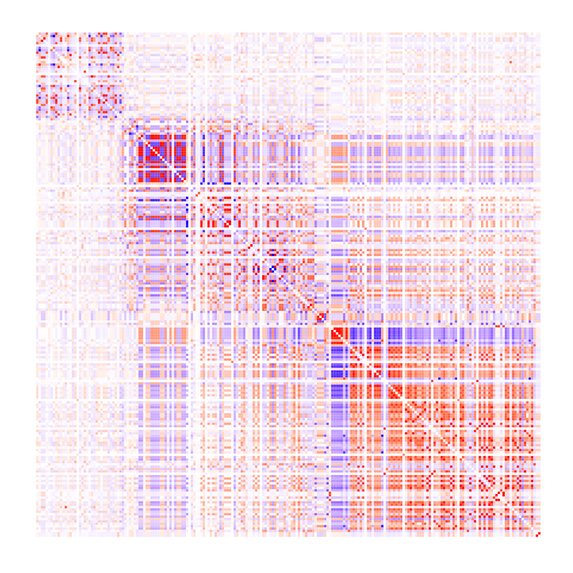
#ggsave(file="docs/figure/computeLD_example.pdf", p1)References
- Lee et al. DISTMIX: direct imputation of summary statistics for unmeasured SNPs from mixed ethnicity cohorts. Bioinformatics. https://doi.org/10.1093/bioinformatics/btv348.
- Lee and Bacanu. GAUSS: a summary-statistics-based R package for accurate estimation of linkage disequilibrium for variants, Gaussian imputation, and TWAS analysis of cosmopolitan cohorts. Bioinformatics. https://doi.org/10.1093/bioinformatics/btae203.