Imputing Z-scores of unmeasured SNPs

Introduction

The growing availability of larger, more ethnically diverse reference panels has increased the need for efficient re-imputation of genotype data and updated GWAS. The GAUSS package streamlines these tasks with its two specialized functions—dist() and distmix()—for imputing association Z-scores for unmeasured SNPs. This vignette will guide you through the practical application of both dist() and distmix() for imputing association Z-scores in both ethnically homogeneous and multi-ethnic cohorts.

Load necessary packages

# Load necessary packages
library(gauss)
library(tidyverse)
library(data.table)
library(kableExtra)

Preparing the Input Data

Both dist() and distmix() functions require two core input datasets:

Association Z-score Data
Reference Panel Data

Association Z-score Data

This data should be in the form of a space-delimited text file including six columns with the following names:

rsid: SNP ID
chr: Chromosome number
bp: Base pair position
a1: Reference allele
a2: Alternative allele
z: Association Z-score

For this example, we will use the Psychiatric Genomic Consortium’s Phase 2 Schizophrenia (PGC SCZ2) GWAS dataset.

# Path to the input file
input_file <- "../data/PGC2_3Mb.txt"

# Input file should include six columns (rsid, chr, bp, a1, a2, and z)
input.data <- fread(input_file, header = TRUE)
head(input.data)
#>          rsid chr        bp a1 a2         z
#> 1:  rs1004467  10 104594507  A  G  6.686674
#> 2:  rs1008013  10 103548866  A  T -1.769923
#> 3: rs10128116  10 103717613  A  G -1.883298
#> 4:  rs1015037  10 105547517  T  G -1.917614
#> 5: rs10159775  10 103184297  A  G  1.304979
#> 6: rs10159838  10 105473937  A  G  2.582526

Reference Panel Data

We will use the 33KG reference panel. Replace the file paths below with those of your actual reference panel files.

reference_index_file <-"../ref/Human/33KG/33kg_index.gz"
reference_data_file <- "../ref/Human/33KG/33kg_geno.gz"
reference_pop_desc_file<-"../ref/Human/33KG/33kg_pop_desc.txt"

The `dist()` function

The dist() function is specifically designed for ethnically homogeneous cohorts. It allows the direct imputation of association Z-scores for unmeasured SNPs, making it easier to update and enhance GWAS analyses.

Arguments

The dist() function accepts following arguments:

chr: Chromosome number.
start_bp: Starting base pair position of the estimation window.
end_bp: Ending base pair position of the estimation window.
wing_size: Size of the area flanking the left and right of the estimation window
study_pop: Study population group
input_file: File name of the association Z-score data
reference_index_file: File name of reference panel index data
reference_data_file: File name of reference panel data
reference_pop_desc_file: File name of reference panel population description data
af1_cutoff: Cutoff of reference allele (a1) frequency

Outputs

The dist() function returns a data frame with following columns:

rsid: SNP ID.
chr: Chromosome number.
bp: Base pair position.
a1: Reference allele.
a2: Alternative allele.
af1ref: Reference allele frequency.
z: Association Z-score.
pval: Association P-value.
info: Imputation information, ranging from 0 to 1.
type: Type of variant. A value of 0 indicates an imputed variant, while 1 denotes a measured variant.

Example Usage

In this example, we will execute the dist() function to impute association Z-scores of missing SNPs in a 1Mb genomic region (Chromosome 10: 104 - 105 Mb) of PGC SCZ2 study. For the sake of this example, let’s assume that the study cohort consists of participants of European descent, represented as “EUR.” Therefore, we’ll set study_pop = "EUR" to utilize genotype data for European subjects from the 33KG reference panel.

af1_cutoff = 0.001

res <- dist(chr=10, 
            start_bp = 104000001, 
            end_bp = 105000000, 
            wing_size = 500000, 
            study_pop = "EUR",
            input_file = input_file, 
            reference_index_file = reference_index_file,
            reference_data_file = reference_data_file, 
            reference_pop_desc_file = reference_pop_desc_file,
            af1_cutoff = af1_cutoff)

Results

head(res) %>% kable("html")

rsid	chr	bp	a1	a2	af1ref	z	pval	info
rs117589665	10	104000008	G	A	0.05720	3.7785313	0.0001578	0.9498775
rs530689457	10	104000125	T	C	0.00336	-1.2757191	0.2020548	0.0831094
rs9664049	10	104000307	T	C	0.61243	-0.4576290	0.6472190	0.9859440
rs149691625	10	104000837	T	C	0.00351	-2.9077590	0.0036403	0.0870822
rs112009583	10	104001402	T	C	0.01793	0.6621509	0.5078745	0.9589020
rs35200058	10	104002372	A	G	0.00575	1.4120431	0.1579373	0.1878804

The `distmix()` function

The distmix() function is designed for multi-ethnic cohorts, extending the capabilities of dist() to accommodate the complexities introduced by ethnic diversity in the data.

Arguments

The distmix() function takes a set of arguments that are largely identical to those for dist(). However, instead of the study_pop argument, distmix() incorporates pop_wgt_df:

pop_wgt_df: An R data frame that specifies the population IDs and their respective ancestry proportions.

Outputs

The output of distmix() is also largely identical to that of dist(), with one exception: the column af1mix replaces af1ref.

af1mix: An estimated reference allele frequency for the variant in the study cohort. It is calculated as a weighted sum of the reference allele frequencies across different populations in the reference panel.

Example Usage

Before using distmix(), you need to prepare ancestry proportion data. This data should be structured as a data frame containing two columns:

pop: Population abbreviation
wgt: Weight or proportion of each population in the study cohort.

You can estimate these proportions using the afmix() function. For a step-by-step guide on this process, refer to the afmix() vignette.

Here, we load pre-generated ancestry proportion data:

# Load the ancestry proportion data
data("PGC2_SCZ_ANC_Prop") # data frame name: PGC2_SCZ_ANC_Prop
head(PGC2_SCZ_ANC_Prop)
#>   pop   wgt
#> 1 ACB 0.006
#> 2 ASW 0.036
#> 3 BEB 0.005
#> 4 CCE 0.008
#> 5 CCS 0.004
#> 6 CDX 0.018

Now, let’s proceed to use distmix() for imputing association Z-scores of missing SNPs in a 1Mb genomic region on Chromosome 10, ranging from 104 to 105 Mb.

af1_cutoff = 0.001

res.mix <- distmix(chr=10, 
            start_bp = 104000001, 
            end_bp = 105000000, 
            wing_size = 500000, 
            pop_wgt_df = PGC2_SCZ_ANC_Prop,
            input_file = input_file, 
            reference_index_file = reference_index_file,
            reference_data_file = reference_data_file, 
            reference_pop_desc_file = reference_pop_desc_file,
            af1_cutoff = af1_cutoff)

Results

head(res.mix) %>% kable("html")

rsid	chr	bp	a1	a2	af1mix	z	pval	info
rs117589665	10	104000008	G	A	0.0498071	3.7654378	0.0001663	0.9502819
rs530689457	10	104000125	T	C	0.0025437	-1.5946868	0.1107823	0.1066830
rs74469897	10	104000130	A	G	0.0019094	-0.3684543	0.7125345	0.0353522
rs115917085	10	104000143	G	T	0.0017765	-0.5972413	0.5503463	0.0405036
rs9664049	10	104000307	T	C	0.6636273	-0.4611097	0.6447199	0.9857300
rs149691625	10	104000837	T	C	0.0046659	-2.7223649	0.0064817	0.0791713

Manhattan Plot

res.mix.info <- res.mix %>% filter(info>0.6)
res.mix.info$type <- factor(res.mix.info$type, 
                            levels=c(0, 1),
                            labels=c("Imputed","Measured"))
gwas.sig <- 5*10^-8
  
ggplot(res.mix.info, aes(x = bp, y = -log10(pval), 
                         color = info, shape=type)) +
  geom_point(alpha = 0.8) +
  geom_hline(aes(yintercept = -log10(gwas.sig)), 
             linetype = "dashed", 
             color = "black", 
             size = 1.5) +
  scale_color_gradient(low = "blue", high = "red") +
  labs(x = "Base Pair Position",
       y = "-Log10(p-value)",
       color = "Info",
       shape = "Type") +
  theme_minimal()
#> Warning: Using `size` aesthetic for lines was deprecated in ggplot2 3.4.0.
#> ℹ Please use `linewidth` instead.

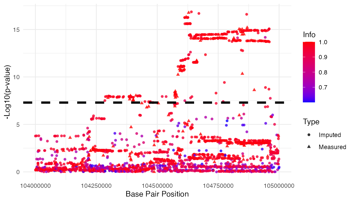
References

Lee et al. DIST: direct imputation of summary statistics for unmeasured SNPs. Bioinformatics . 2013 Nov 15;29(22):2925-7. doi: 10.1093/bioinformatics/btt500.
Lee et al. DISTMIX: direct imputation of summary statistics for unmeasured SNPs from mixed ethnicity cohorts. Bioinformatics. https://doi.org/10.1093/bioinformatics/btv348

Introduction

Load necessary packages

Preparing the Input Data

Association Z-score Data

Reference Panel Data

The dist() function

Arguments

Outputs

Example Usage

Results

The distmix() function

Arguments

Outputs

Example Usage

Results

Manhattan Plot

References

The `dist()` function

The `distmix()` function